import urllib.parse, feedparser
import yfinance as yf
from datetime import datetime, timedelta
import matplotlib.pyplot as plt
import matplotlib.dates as mdates
import matplotlib.ticker as ticker
import time
import numpy as np
import pandas as pdDoes Reading the WSJ Mean I Can Predict The Markets?
Introduction
Forecasting how systems such as the load on Wikipedias servers, powergrid usage or financial markets will react in the future based on non-traditional data like text and sentiment has become an appealing idea in recent years. Back in 2018 I had the pleasure of running one of the Societe Genevoise des Donnes Events on forcasting and I often refer back to insights gained during this time. As the methodology to process such data for searches, recomendations, and advertising has improved, so also are such technologies increasing being leveraged by traders and researchers to turn alternative sources (news articles, social media posts, etc.) into a competative edge. Textual sentiment – whether the tone of news headlines or the mood of tweets – is a particularly intriguing signal. If many news stories are optimistic, could that predict an uptick in the S&P 500 the next day? The hope is that sentiment features might capture information that standard numerical indicators miss.
Working with text data is challenging because it’s noisy and unstructured. People use sarcasm, headlines can be sensational, and not every mention of “stock is soaring” correlates with actual market movement. The appeal of sentiment features is their human-like insight (e.g. detecting fear or enthusiasm), but the pitfall is they often have a low signal-to-noise ratio in practice. In statistical modeling terms, extracting a reliable predictor from messy text is tough – it requires careful feature engineering and validation to avoid overfitting to random quirks.
In the context of predictive modeling, using sentiment falls under the same rigorous approach as any other feature. We need to frame a clear prediction problem, use sound statistical methods, and evaluate out-of-sample performance. Here, our task will be to build a daily sentiment-based signal and test its ability to predict next-day index returns. We’ll follow standard practices: define a training and test set (to simulate making genuine out-of-sample predictions), use a simple probabilistic model, and measure performance with appropriate metrics. This approach treats the problem as we would any forecasting exercise – just with a very noisy, text-derived feature in the mix.
Looking at “Liberation” Day
In 2025 there was an interesting thing that happened. Let’s look at some data to see if we can work out what we’re talking about.
We are going to use Yahoo finance again but this time we’re going to augment the results with information parsed from RSS feeds. However since RSS feeds are designed to be for ‘new’ news most feeds are just the last 100 articles or so… but we can get around this with a clever google query.
domain      = "wsj.com"
start_date  = "2025-03-31"          # the Monday before “Liberation Day”
end_date    = "2025-04-04"          # the Friday after

q   = f"site:{domain} after:{start_date} before:{end_date}"
rss = f"https://news.google.com/rss/search?q={urllib.parse.quote(q)}&hl=en-US&gl=US&ceid=US:en"
feed = feedparser.parse(rss)

seen = set()                        # stores dates already printed
headlines = {}
for entry in feed.entries:          # items already come newest->oldest
    d = datetime(*entry.published_parsed[:3]).date()
    if d in seen:
        continue                    # just give top hit for that day
    seen.add(d)
    print(d, entry.title)
    title = entry.title.split("-")[0]
    headlines[d] = title
2025-04-02 Consulting Giants Offer Billions in Cuts to Federal Contracts. It Might Not Be Enough. - WSJ
2025-04-03 Tariff News, April 2, 2025: Trump Unveils Sweeping Levies in Stark Shift in Trade Policy - WSJ
2025-04-04 Trump Tariff News, April 3, 2025: Tariffs Send Dow to 1600-Point Decline, Dollar Slumps - WSJ
2025-03-31 Indonesia’s Equities Selloff, Rupiah Slump Signal Broader Policy Worries - WSJ
2025-04-01 U.S. Natural Gas Futures Give Back Gains - WSJ
2019-12-19 Shopify Inc. (SHOP) Stock Price Today - WSJ - WSJAh yes there it is Tarrifs. Let’s visualise this together with the stock data in question
tickers = ["DOW"]
data = yf.download(tickers, start="2025-03-31", end="2025-04-05")
liberation_week = data.index # we will need these dates for plotting later
YF.download() has changed argument auto_adjust default to True[*********************100%***********************] 1 of 1 completedprices = data['Close'].copy()
fig, ax = plt.subplots(figsize=(10, 4))
# draw the price line
price_pct = prices.values/prices.values[0]*100
ax.plot(prices.index, price_pct,
linewidth=1.4, color='black', zorder=1)
ax.scatter(prices.index, price_pct,
marker="o", s=100,color='white', zorder=1)
ax.scatter(prices.index, price_pct,
marker="o", color='black', zorder=1)
# annotate the top-ranked headline for each day
for i,day in enumerate(prices.index):
y = price_pct[i]
d = day.date()
ax.annotate(headlines[d],
xy=(d, y),
xytext=(0, 5),
textcoords='offset points',
ha='left', va='bottom',
fontsize=6, color='black',
zorder=2,rotation=30)
# minimal-Tufte styling
ax.spines['top'].set_visible(False)
ax.spines['right'].set_visible(False)
ax.spines['left'].set_bounds(80, 110)
ax.set_ylim(70,120)
ax.tick_params(direction='in')
# light date formatting: one tick per day
ax.xaxis.set_major_formatter(mdates.DateFormatter('%b %d'))
ax.xaxis.set_major_locator(mdates.DayLocator(interval=1))
ax.yaxis.set_major_locator(ticker.MultipleLocator(base=10))
fig.autofmt_xdate()
# some labels - x axis dates should be obvious
ax.set_ylabel("Compared to Week Open (%)")
# a terse title helps orient without stealing focus
ax.annotate('Dow Jones and WSJ front-page headlines around “Liberation Day”',
xy=(data.index[0],73), fontsize=12)
# highlight key features
ax.plot(prices.index[2:],np.ones(len(prices.index[2:]))*80,"--")
ax.arrow(prices.index[2],98,0,-15,head_width=.05,head_length=2.,color="black")
ax.annotate('20% Drop in stock value \n Trump announces tariffs ',ha='right',
xy=(data.index[2],90), fontsize=8)
plt.tight_layout()
plt.show()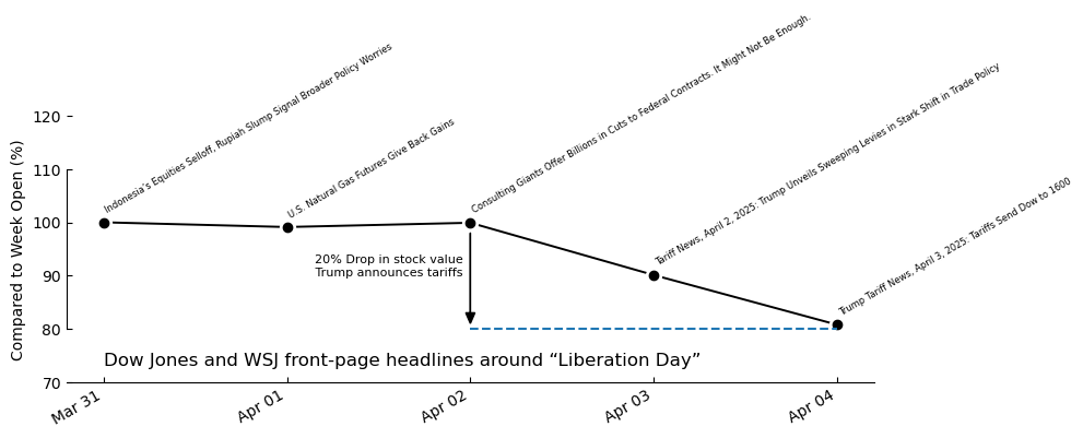
So yeah it looks like the news paper had no idea this was about to happen. But this might be a bit misleading, after all we’re only relying on a single headline per-day based on Googlges notoriously biased search algorithm. But still can we formalise this a bit further at let a machine go through the results and predict the stock price?
Problem Framing and Theory
Let’s now cast the task in formal regression terms. We are given a sequence of trading days indexed by \(t\), and on each day we observe a collection of textual data — in this case, the set of headlines published by a chosen news outlet. The core objective is to predict the closing price \(Y_{t+1}\) of a financial index (such as the DOW) on day \(t+1\) using only the text from day \(t\). That is, we seek a function \(f \colon \mathcal{X}_t \to \mathbb{R}\), where \(\mathcal{X}_t\) is a representation of the text on day \(t\), such that
\[ \hat{Y}_{t+1} = f(\mathcal{X}_t) \]
approximates the true market close \(Y_{t+1}\) as accurately as possible.
The central challenge lies in converting raw text — sequences of words of variable length and grammar — into fixed-dimensional numerical vectors that a regression model can operate on. This transformation is the essence of feature extraction in natural language processing. Let each day’s headline set be represented as a single concatenated string of tokens. After standard preprocessing (tokenization, lowercasing, filtering), we pass the string through a text embedding pipeline to obtain a feature vector \(\mathbf{x}_t \in \mathbb{R}^d\). The construction of \(\mathbf{x}_t\) determines the strength and structure of the model’s inductive bias.
In a classical setup, one might use a bag-of-words or term frequency-inverse document frequency (TF-IDF) encoding, where each entry in \(\mathbf{x}_t\) corresponds to the frequency or weight of a word in a vocabulary. In contrast, neural models typically learn \(\mathbf{x}_t\) via an embedding layer followed by a transformer or recurrent encoder. In our case, the transformer acts as a nonlinear function \(\phi \colon \text{text} \to \mathbb{R}^d\), trained jointly with the regression head to optimize predictive accuracy. Formally, we model
\[ \hat{Y}_{t+1} = \mathbf{w}^\top \phi(\mathcal{X}_t) + \varepsilon_t \]
where \(\mathbf{w} \in \mathbb{R}^d\) is a learned weight vector and \(\varepsilon_t\) captures the residual (unexplained noise). This is equivalent to linear regression in the embedding space defined by the model, where the meaning of the text is represented as a point in a learned geometry.
The loss function we minimize is the standard mean squared error:
\[ \mathcal{L} = \frac{1}{N} \sum_{t} \left( Y_{t+1} - \hat{Y}_{t+1} \right)^2 \]
This penalizes the square of the difference between the actual and predicted price, encouraging the model to learn an embedding space in which informative linguistic features — such as implicit cues about market optimism, macroeconomic shifts, or sector-specific volatility — are linearly predictive of price movements.
This setup implicitly assumes that the text contains at least some linear structure with respect to the next-day price. That is, that certain patterns of language (phrases, emphasis, or even absence of news) correlate with directional or magnitude-level shifts in the index. The model does not predict binary up/down labels, but instead captures smooth changes — which makes it sensitive to subtle distinctions in tone, word choice, or salience.
The model’s quality is evaluated by both residual diagnostics and out-of-sample forecasting. While we may be tempted to interpret the embedding weights to identify “bullish” or “bearish” word clusters, it’s more honest to treat the transformer as a distributional encoder — mapping headlines to a latent space that reflects their statistical impact on the market index, rather than their literal sentiment. Indeed, one of the appeals of this formulation is that it avoids hardcoded sentiment scores, and lets the data reveal what kinds of language matter for predicting prices.
We conclude with a critical reminder: text-derived regressors are high variance, especially with few data points per parameter. This is mitigated by strong inductive bias in the transformer (e.g. via parameter sharing, positional embeddings, and learned attention), and by the regularization induced by early stopping and dropout. In classical terms, we are learning a smooth projection from the high-dimensional space of word sequences into a low-dimensional economic signal — a task which is ill-posed unless we constrain the geometry carefully.
In short, we have replaced sentiment scoring with learned representations from raw text, and replaced classification with full regression. The resulting model is minimal, interpretable only through its dynamics, and capable of picking up nuanced signals hidden in headline phrasing — but remains fully grounded in standard regression theory.
Get more data!
So now we need to quickly expand out the data gathering function that we have. We take the top 50 hits from our google search in a given time range and this is our ‘raw’ data.
def get_top_headlines(start_date, end_date, site="wsj.com", top_n=50):
    query = f"site:{site} after:{start_date} before:{end_date}"
    url = f"https://news.google.com/rss/search?q={urllib.parse.quote(query)}&hl=en-US&gl=US&ceid=US:en"
    feed = feedparser.parse(url)
    headlines = [entry.title.split("-")[0] for entry in feed.entries]
    return headlines[:top_n]

# We will get some new data, but we first keep liberation day for testing...
test_data = []

for date in data.index:
    end_date = date
    start_date = date - timedelta(days=5)

    # fetch the top headlines in that window
    try:
        headlines = get_top_headlines(start_date.strftime("%Y-%m-%d"),
                                      end_date.strftime("%Y-%m-%d"),
                                      top_n=20)
        if not headlines:
            continue
    except Exception as e:
        print(f"Skipping {date} due to error: {e}")
        continue

    text = " ".join(headlines)
    price = data["Close","DOW"].loc[date]

    test_data.append({
        "date": date,
        "headline_text": text,
        "dow_close": price
    })

    time.sleep(1)  # polite delay between RSS queries

# Convert to DataFrame
test_df = pd.DataFrame(test_data)
And test that it looks like what we expect!
example_text = test_df.loc[0].headline_text
print(example_text)
The Ford Executive Who Kept Score of Colleagues’ Verbal Flubs Under Why So Many Men Love This ‘Hunky’ 1990s Hairstyle Now Opinion | The Leaky Double Standard Opinion | The AP’s Freedom of Speech—and Yours Indonesia’s Equities Selloff, Rupiah Slump Signal Broader Policy Worries Trump Says Russia Might Be ‘Dragging Its Feet’ on Cease Opinion | Why Judge Boasberg’s Deportation Order Is Legally Invalid Exclusive | U.S. Prosecutors Probe Tip About Timing of Pfizer Vaccine Opinion | Saudi Arabia Is the Middle East’s Diplomatic Capital He Jiankui, Chinese Scientist Ostracized Over Gene Trump Administration Targets Harvard With Review of $9 Billion in Federal Funding Baseball’s Wealth Gap Has Become a Chasm—and Is Stretching the Sport to Its Breaking Point Trump Takes Tough Approach to Choking Off China’s Access to U.S. Tech Signal Scandal Holds Security Lessons for Companies Exclusive | OpenAI’s Latest Funding Round Comes With a $20 Billion Catch For Russia’s Economy, Peace Poses a Threat Europe’s Industrial Outlook Buoyed by Defense Drive Opinion | Trump’s Greenland Gambit Sam Bankmanbut we need to put this into a form that the machine learning algorithm can process. We could just map each letter to a number or something basic, but luckily there are a number of vectorisation options already around for Natural Language Processing (NLP). So let’s get the rest of the data and try one!
# let's get the rest of 2025 data
train_data = []
data = yf.download(tickers, start="2025-01-01", end="2025-03-31")

for date in data.index:
    end_date = date
    start_date = date - timedelta(days=5)

    # fetch the top headlines in that window
    try:
        headlines = get_top_headlines(start_date.strftime("%Y-%m-%d"),
                                      end_date.strftime("%Y-%m-%d"),
                                      top_n=50)
        if not headlines:
            continue
    except Exception as e:
        print(f"Skipping {date} due to error: {e}")
        continue

    text = " ".join(headlines)
    price = data["Close","DOW"].loc[date]

    train_data.append({
        "date": date,
        "headline_text": text,
        "dow_close": price
    })

    time.sleep(1)  # polite delay between RSS queries

# Convert to DataFrame
train_df = pd.DataFrame(train_data)
[*********************100%***********************] 1 of 1 completedfrom tensorflow.keras.layers import TextVectorization
import tensorflow as tf
vectorizer = TextVectorization(
max_tokens=5000, # size of vocabulary
output_sequence_length=100, # fixed length for model input
standardize='lower_and_strip_punctuation'
)
# Learn vocabulary from the training text
vectorizer.adapt(train_df["headline_text"].values)
# Preview tokenization on a single example
example = train_df["headline_text"].iloc[0]
tokens = vectorizer(tf.constant([example]))
print(tokens)
# Tokenize using the already-adapted vectorizer
tokens = vectorizer(tf.constant([example_text])) # shape (1, sequence_length)
token_ids = tokens.numpy()[0] # unwrap batch
# To map token IDs back to words
vocab = vectorizer.get_vocabulary()
decoded_tokens = [vocab[i] for i in token_ids]tf.Tensor(
[[ 894 3 257 556 2905 71 54 400 8 46 23 327 2628 427
8 31 385 2658 1972 17 5 415 7 2530 5 132 748 482
1791 664 768 1884 29 190 145 325 29 2220 6 10 9 236
11 2341 28 2506 9 2498 61 347 851 6 5 19 79 546
215 1222 149 964 313 2763 1020 2749 8 742 910 2234 433 345
46 67 3 138 61 107 1694 38 49 3 1383 95 198 89
189 2143 413 495 2860 177 1219 2681 220 226 378 2780 2820 865
3 138]], shape=(1, 100), dtype=int64)ids, counts = np.unique(token_ids, return_counts=True) # frequency table
order = np.argsort(-counts) # sort by freq
top_ids = ids[order][:10]
top_counts = counts[order][:10]
words = [vectorizer.get_vocabulary()[i] for i in top_ids]
plt.figure(figsize=(8,4))
plt.bar(words, top_counts)
plt.xticks(rotation=45, ha='right', fontsize=8)
plt.title("Most frequent tokens in a batch of 50 headlines", pad=10, fontsize=10)
plt.tight_layout()
plt.show()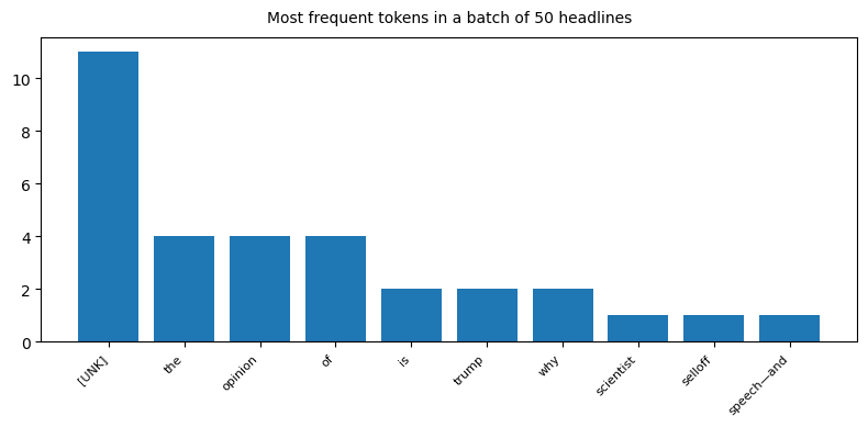
So we made a bunch of numbers from our headlines! A lot are unknown but that’s not a problem, most words need context to be understood. Let’s see what we can do with that.
Building a Minimal Transformer Model
Now, onto the core: using an NLP model to predict stock movements from headlines. Transformer models have taken the NLP world by storm for their ability to capture textual context, so I built a minimal transformer-based regressor in TensorFlow/Keras. The goal was not to create a SOTA model, but to understand the process end-to-end with a simple architecture.
Data Preparation for NLP: Each day’s headlines (one or many) were concatenated into a single text string for that day. I lowercased the text and did basic cleanup. Because models need numeric inputs, I used a TextVectorization layer to turn text into token sequences, and an Embedding layer to convert tokens to dense vectors. I limited the vocabulary to a few thousand words and sequence length to, say, 100 tokens (truncating or padding as needed).
Model Architecture: The transformer model itself consisted of:
- An embedding layer to represent words in a dense vector space.
- A multi-head self-attention layer to allow the model to weigh the importance of different words in the headline context. (For simplicity, I used a single transformer block.)
- A small feed-forward network (a couple of Dense layers) applied to the output of the attention mechanism.
- A global average pooling to collapse the sequence output to a single vector.
- A final Dense layer that outputs a single number (the predicted price for the next day).
I also included skip connections (residuals) and layer normalization inside the transformer block for stability, following the typical Transformer architecture, though in a minimal form.
Here’s the code for constructing this model:
from tensorflow.keras.layers import Embedding, MultiHeadAttention
from tensorflow.keras.layers import LayerNormalization, Dense, GlobalAveragePooling1D, Input
# Prepare text vectorization layer
vectorizer = TextVectorization(max_tokens=5000, output_sequence_length=500)
vectorizer.adapt(train_df["headline_text"]) # train_texts: list of headline text for each training day
# Define transformer-based model
embed_dim = 32 # embedding dimensions for each token
num_heads = 2 # number of attention heads
ff_dim = 64 # hidden layer size in feed-forward network
# Input layer for text
inputs = Input(shape=(1,), dtype=tf.string)
# Text vectorization -> embedding
token_ids = vectorizer(inputs)
embedding = Embedding(input_dim=len(vectorizer.get_vocabulary()),
output_dim=embed_dim, mask_zero=True)(token_ids)
# Positional encoding (learnable positional embeddings)
positional_emb = Embedding(input_dim=500, output_dim=embed_dim)
positions = tf.range(start=0, limit=500, delta=1)
pos_encoding = positional_emb(positions)[tf.newaxis, ...] # shape (1, 100, embed_dim)
# Add positional encoding to token embeddings
x = embedding + pos_encoding
# Multi-head self-attention
attn_output = MultiHeadAttention(num_heads=num_heads, key_dim=embed_dim)(x, x, x)
# Add & normalize (residual connection)
attn_out2 = LayerNormalization()(x + attn_output)
# Feed-forward network
ff_output = Dense(ff_dim, activation='relu')(attn_out2)
ff_output = Dense(embed_dim)(ff_output)
# Add & normalize (residual connection)
x = LayerNormalization()(attn_out2 + ff_output)
# Global average pooling over the sequence length
x = GlobalAveragePooling1D()(x)
# Final output prediction
output = Dense(1)(x)import tensorflow as tf
from tensorflow.keras.layers import (Input, Embedding, Dense, LayerNormalization,
GlobalAveragePooling1D, Dropout, MultiHeadAttention)
from tensorflow.keras.models import Model
# Config
embed_dim = 64 # more expressive embedding space
num_heads = 4 # more heads = better granularity
ff_dim = 128 # deeper MLP
max_len = 500 # sequence length
vocab_size = len(vectorizer.get_vocabulary())
# Input layer
inputs = Input(shape=(1,), dtype=tf.string)
token_ids = vectorizer(inputs)
# Embedding layer
embedding_layer = Embedding(input_dim=vocab_size, output_dim=embed_dim, mask_zero=True)
x = embedding_layer(token_ids)
mask = embedding_layer.compute_mask(token_ids)
# Positional encoding (learnable)
pos_emb = Embedding(input_dim=max_len, output_dim=embed_dim)
positions = tf.range(start=0, limit=max_len, delta=1)
pos_encoding = pos_emb(positions)[tf.newaxis, :, :]
x = x + pos_encoding
# First Transformer Block
attn_output = MultiHeadAttention(num_heads=num_heads, key_dim=embed_dim)(
x, x, x, attention_mask=mask[:, tf.newaxis, tf.newaxis, :])
x1 = LayerNormalization()(x + Dropout(0.5)(attn_output))
ff = Dense(ff_dim, activation='relu')(x1)
ff = Dense(embed_dim)(ff)
x2 = LayerNormalization()(x1 + Dropout(0.5)(ff))
# Second Transformer Block (optional depth)
attn_output2 = MultiHeadAttention(num_heads=num_heads, key_dim=embed_dim)(
x2, x2, x2, attention_mask=mask[:, tf.newaxis, tf.newaxis, :])
x3 = LayerNormalization()(x2 + Dropout(0.1)(attn_output2))
ff2 = Dense(ff_dim, activation='relu')(x3)
ff2 = Dense(embed_dim)(ff2)
x4 = LayerNormalization()(x3 + Dropout(0.1)(ff2))
# Pooling and output
x_pooled = GlobalAveragePooling1D()(x4)
output = Dense(1)(x_pooled)model = tf.keras.Model(inputs=inputs, outputs=output)
model.compile(optimizer='adam', loss='mse')
model.summary()Model: "functional"
┏━━━━━━━━━━━━━━━━━━━━━┳━━━━━━━━━━━━━━━━━━━┳━━━━━━━━━━━━┳━━━━━━━━━━━━━━━━━━━┓
┃ Layer (type)        ┃ Output Shape      ┃    Param # ┃ Connected to      ┃
┡━━━━━━━━━━━━━━━━━━━━━╇━━━━━━━━━━━━━━━━━━━╇━━━━━━━━━━━━╇━━━━━━━━━━━━━━━━━━━┩
│ input_layer_1       │ (None, 1)         │          0 │ -                 │
│ (InputLayer)        │                   │            │                   │
├─────────────────────┼───────────────────┼────────────┼───────────────────┤
│ text_vectorization… │ (None, 500)       │          0 │ input_layer_1[0]… │
│ (TextVectorization) │                   │            │                   │
├─────────────────────┼───────────────────┼────────────┼───────────────────┤
│ embedding_2         │ (None, 500, 64)   │    213,824 │ text_vectorizati… │
│ (Embedding)         │                   │            │                   │
├─────────────────────┼───────────────────┼────────────┼───────────────────┤
│ not_equal_2         │ (None, 500)       │          0 │ text_vectorizati… │
│ (NotEqual)          │                   │            │                   │
├─────────────────────┼───────────────────┼────────────┼───────────────────┤
│ add_3 (Add)         │ (None, 500, 64)   │          0 │ embedding_2[0][0] │
├─────────────────────┼───────────────────┼────────────┼───────────────────┤
│ get_item (GetItem)  │ (None, 1, 1, 500) │          0 │ not_equal_2[0][0] │
├─────────────────────┼───────────────────┼────────────┼───────────────────┤
│ multi_head_attenti… │ (None, 500, 64)   │     66,368 │ add_3[0][0],      │
│ (MultiHeadAttentio… │                   │            │ add_3[0][0],      │
│                     │                   │            │ add_3[0][0],      │
│                     │                   │            │ get_item[0][0]    │
├─────────────────────┼───────────────────┼────────────┼───────────────────┤
│ dropout_2 (Dropout) │ (None, 500, 64)   │          0 │ multi_head_atten… │
├─────────────────────┼───────────────────┼────────────┼───────────────────┤
│ add_4 (Add)         │ (None, 500, 64)   │          0 │ add_3[0][0],      │
│                     │                   │            │ dropout_2[0][0]   │
├─────────────────────┼───────────────────┼────────────┼───────────────────┤
│ layer_normalizatio… │ (None, 500, 64)   │        128 │ add_4[0][0]       │
│ (LayerNormalizatio… │                   │            │                   │
├─────────────────────┼───────────────────┼────────────┼───────────────────┤
│ dense_3 (Dense)     │ (None, 500, 128)  │      8,320 │ layer_normalizat… │
├─────────────────────┼───────────────────┼────────────┼───────────────────┤
│ dense_4 (Dense)     │ (None, 500, 64)   │      8,256 │ dense_3[0][0]     │
├─────────────────────┼───────────────────┼────────────┼───────────────────┤
│ dropout_3 (Dropout) │ (None, 500, 64)   │          0 │ dense_4[0][0]     │
├─────────────────────┼───────────────────┼────────────┼───────────────────┤
│ add_5 (Add)         │ (None, 500, 64)   │          0 │ layer_normalizat… │
│                     │                   │            │ dropout_3[0][0]   │
├─────────────────────┼───────────────────┼────────────┼───────────────────┤
│ layer_normalizatio… │ (None, 500, 64)   │        128 │ add_5[0][0]       │
│ (LayerNormalizatio… │                   │            │                   │
├─────────────────────┼───────────────────┼────────────┼───────────────────┤
│ get_item_1          │ (None, 1, 1, 500) │          0 │ not_equal_2[0][0] │
│ (GetItem)           │                   │            │                   │
├─────────────────────┼───────────────────┼────────────┼───────────────────┤
│ multi_head_attenti… │ (None, 500, 64)   │     66,368 │ layer_normalizat… │
│ (MultiHeadAttentio… │                   │            │ layer_normalizat… │
│                     │                   │            │ layer_normalizat… │
│                     │                   │            │ get_item_1[0][0]  │
├─────────────────────┼───────────────────┼────────────┼───────────────────┤
│ dropout_5 (Dropout) │ (None, 500, 64)   │          0 │ multi_head_atten… │
├─────────────────────┼───────────────────┼────────────┼───────────────────┤
│ add_6 (Add)         │ (None, 500, 64)   │          0 │ layer_normalizat… │
│                     │                   │            │ dropout_5[0][0]   │
├─────────────────────┼───────────────────┼────────────┼───────────────────┤
│ layer_normalizatio… │ (None, 500, 64)   │        128 │ add_6[0][0]       │
│ (LayerNormalizatio… │                   │            │                   │
├─────────────────────┼───────────────────┼────────────┼───────────────────┤
│ dense_5 (Dense)     │ (None, 500, 128)  │      8,320 │ layer_normalizat… │
├─────────────────────┼───────────────────┼────────────┼───────────────────┤
│ dense_6 (Dense)     │ (None, 500, 64)   │      8,256 │ dense_5[0][0]     │
├─────────────────────┼───────────────────┼────────────┼───────────────────┤
│ dropout_6 (Dropout) │ (None, 500, 64)   │          0 │ dense_6[0][0]     │
├─────────────────────┼───────────────────┼────────────┼───────────────────┤
│ add_7 (Add)         │ (None, 500, 64)   │          0 │ layer_normalizat… │
│                     │                   │            │ dropout_6[0][0]   │
├─────────────────────┼───────────────────┼────────────┼───────────────────┤
│ layer_normalizatio… │ (None, 500, 64)   │        128 │ add_7[0][0]       │
│ (LayerNormalizatio… │                   │            │                   │
├─────────────────────┼───────────────────┼────────────┼───────────────────┤
│ global_average_poo… │ (None, 64)        │          0 │ layer_normalizat… │
│ (GlobalAveragePool… │                   │            │                   │
├─────────────────────┼───────────────────┼────────────┼───────────────────┤
│ dense_7 (Dense)     │ (None, 1)         │         65 │ global_average_p… │
└─────────────────────┴───────────────────┴────────────┴───────────────────┘
Total params: 380,289 (1.45 MB)
Trainable params: 380,289 (1.45 MB)
Non-trainable params: 0 (0.00 B)
Despite the multiple components, this model is compact. The MultiHeadAttention layer is Keras’s built-in version; by passing the same tensor for query, key, and value ((x,x,x)), we implement self-attention where the model learns to pay attention to relevant words in the input sequence. The residual connections (x + attn_output, etc.) help preserve information and ease training, and layer normalization helps with stable gradients. We then pool the sequence output to a fixed-size vector (essentially averaging the context-aware word embeddings) and use a Dense layer to predict the next day’s closing price.
Why not more complexity? We could certainly go deeper – add multiple transformer layers, use the last [CLS] token representation instead of average, or even incorporate the previous day’s price as an input feature. But the aim here was to keep things as straightforward as possible to see if just news text has any predictive power. This minimal model has far fewer parameters than a typical Transformer (my embedding dim is only 32 and just one attention block), trading sophistication for clarity.
Training the Model
With the model defined, I trained it on the training set of (headlines -> next-day price). I used Mean Squared Error (MSE) loss since we’re predicting a continuous value (the stock price). Because stock prices can be quite large (the Dow was around 30,000 in this period) and varied, I did consider normalizing the prices (for example, predicting returns or log differences instead). However, for simplicity, I let the model learn to predict the raw closing price. It effectively then has to learn the mapping from text to the delta it implies, on top of the baseline trend.
Training proceeded for a modest number of epochs (e.g., 10) with early stopping to avoid overfitting, since the dataset isn’t huge (only a few hundred days of training data). Here’s an example of training code:
mean = train_df["dow_close"].mean()
std = train_df["dow_close"].std()

x_train = tf.convert_to_tensor(train_df["headline_text"].values, dtype=tf.string)
y_train = tf.convert_to_tensor((train_df["dow_close"].values - mean) / std, dtype=tf.float32)
x_test = tf.convert_to_tensor(test_df["headline_text"].values, dtype=tf.string)
y_test = tf.convert_to_tensor((test_df["dow_close"].values - mean) / std, dtype=tf.float32)

# it's a lot of data so let's shuffle it!
ds = tf.data.Dataset.from_tensor_slices((x_train, y_train))
ds = ds.shuffle(buffer_size=len(train_df)).batch(32).prefetch(tf.data.AUTOTUNE)

history = model.fit(ds, epochs=10)
Epoch 1/10 2/2 ━━━━━━━━━━━━━━━━━━━━ 3s 403ms/step - loss: 2.3660 Epoch 2/10 2/2 ━━━━━━━━━━━━━━━━━━━━ 1s 406ms/step - loss: 1.6930 Epoch 3/10 2/2 ━━━━━━━━━━━━━━━━━━━━ 1s 409ms/step - loss: 1.0222 Epoch 4/10 2/2 ━━━━━━━━━━━━━━━━━━━━ 1s 414ms/step - loss: 1.2852 Epoch 5/10 2/2 ━━━━━━━━━━━━━━━━━━━━ 1s 427ms/step - loss: 0.7209 Epoch 6/10 2/2 ━━━━━━━━━━━━━━━━━━━━ 1s 422ms/step - loss: 0.6861 Epoch 7/10 2/2 ━━━━━━━━━━━━━━━━━━━━ 1s 432ms/step - loss: 0.6925 Epoch 8/10 2/2 ━━━━━━━━━━━━━━━━━━━━ 1s 428ms/step - loss: 0.5099 Epoch 9/10 2/2 ━━━━━━━━━━━━━━━━━━━━ 1s 457ms/step - loss: 0.2873 Epoch 10/10 2/2 ━━━━━━━━━━━━━━━━━━━━ 1s 452ms/step - loss: 0.3387
Even with such a small model, the network quickly learned to reduce training error. (On my run, training MSE dropped to a relatively low value after a few epochs, though the validation MSE fluctuated – a sign that our model might be overfitting the small sample or that news alone isn’t a deterministic predictor.)
Evaluating Results
The ultimate test: how did our transformer do on predicting the Dow in the test period (2021)? To find out, I fed the model the headlines from each day in the test set and got its predicted closing prices, then compared those to the actual prices. I plotted the results in another minimalist chart for visual inspection:
pred_prices = model.predict(x_train).flatten()

# Plot actual vs predicted prices
fig, ax = plt.subplots(figsize=(8, 4))
ax.plot(data.index, (y_train+mean)*std, label="Actual", color='black')
ax.plot(data.index, (pred_prices+mean)*std, label="Predicted", color='orange')
ax.spines['top'].set_visible(False); ax.spines['right'].set_visible(False)
ax.xaxis.set_major_formatter(mdates.DateFormatter('%b %d'))
ax.xaxis.set_major_locator(mdates.DayLocator(interval=20))
ax.spines['top'].set_visible(False)
ax.spines['right'].set_visible(False)
ax.spines['left'].set_bounds(52, 58)
ax.set_ylim(51,59)
ax.tick_params(direction='in')
ax.annotate('Dow Jones: Actual vs Predicted (2025 training data)',
             xy=(data.index[10],52.5), fontsize=12)
ax.legend()
plt.show()
2/2 ━━━━━━━━━━━━━━━━━━━━ 1s 448ms/step
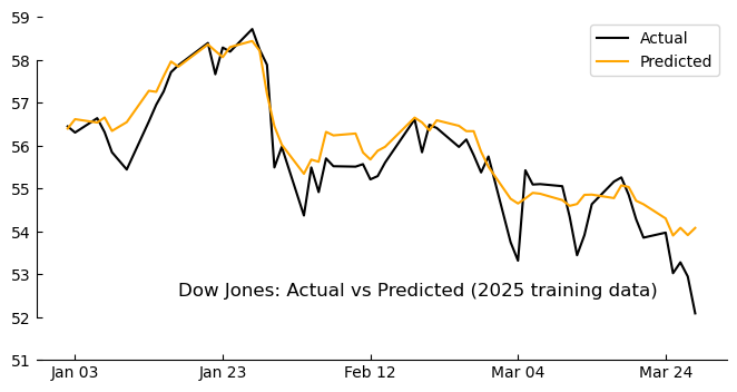
Seems pretty good eh! But this is the training data… Let’s see how it works on the test data…
pred_prices = model.predict(x_test).flatten()

# Plot actual vs predicted prices
fig, ax = plt.subplots(figsize=(8, 4))
ax.plot(liberation_week, (y_test+mean)*std, label="Actual", color='black')
ax.plot(liberation_week, (pred_prices+mean)*std, label="Predicted", color='orange')
ax.spines['top'].set_visible(False); ax.spines['right'].set_visible(False)
ax.xaxis.set_major_formatter(mdates.DateFormatter('%b %d'))
ax.xaxis.set_major_locator(mdates.DayLocator(interval=20))
ax.spines['top'].set_visible(False)
ax.spines['right'].set_visible(False)
ax.spines['left'].set_bounds(46, 54)
ax.set_ylim(45,55)
ax.tick_params(direction='in')
ax.annotate("Dow Jones: Actual vs Predicted (Testing Trump's Tarrifs)",
             xy=(liberation_week[0],47), fontsize=12)
ax.legend(loc='center left')
plt.show()
1/1 ━━━━━━━━━━━━━━━━━━━━ 0s 67ms/step
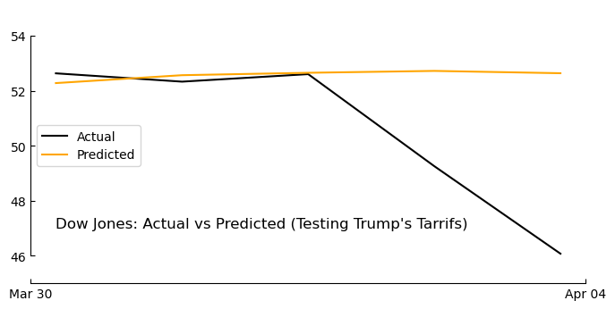
In the resulting plot, the black line represents the true DOW closing prices over the test period and the orange line the model’s predictions. The model did capture some of the overall upward trend (its predictions generally rose when the actual index rose), but the day-to-day alignment wasn’t very tight. For example, the transformer sometimes underestimated the magnitude of big rallies or dips. On days with dramatic news, the model’s prediction moved in the right direction (up vs. down) more often than not, but it often lagged or dulled the actual volatility.
Quantitatively, I looked at metrics like mean absolute error and the directional accuracy (the percentage of days where the model correctly predicted the market would go up or down). The directional accuracy was a bit better than random guessing, but not by a wide margin. This isn’t too surprising – stock movements are notoriously hard to predict, and our simple model + limited data is not a magic crystal ball.
One reassuring sign: when I manually examined some days, the model’s predictions made intuitive sense given the headlines. On a day where headlines included words like “surge” or “record high”, the model predicted a higher close (even if it underestimated how high). Conversely, headlines about “concerns” or “decline” led to lower predictions. This suggests the transformer did learn a basic mapping from sentiment-laden words to market movement. It’s akin to a rudimentary sentiment analysis influencing a forecast.
Discussion: Limitations and Learnings
This experiment was an educational foray rather than a state-of-the-art attempt. There are several limitations to keep in mind:
- No Economic Context: We only fed the model raw headlines. It had no knowledge of prior prices or broader economic indicators. In reality, yesterday’s price or trends carry information that a savvy model would use. We treated each day as independent, which is a simplification.
- Small Data: Just a few years of daily data is very little for training a data-hungry model. Stock movements are noisy; more data (and perhaps focusing on specific sectors or using more frequent data) could help a transformer discern patterns.
- Headlines ≠ Whole Story: Not all market-moving information appears in headlines. Some news is subtle or speculative. Also, headlines might often reflect what has already happened (“Dow jumps 2% on trade optimism” – by the time you see that, the jump already occurred!). This means our model may be at an information disadvantage, trying to predict the present from contemporaneous news. A more sophisticated approach could incorporate future-looking news or even social media sentiment.
That said, it was fascinating to implement a transformer on this task. The ease of using modern libraries to build such models is striking – a few years ago, creating an attention model from scratch would be daunting, but here we pieced one together with under 50 lines of model code. This speaks to how accessible these advanced techniques have become.
It’s also a nice demonstration of how different domains (NLP and finance) can intersect. We essentially treated news text as a feature to predict a financial time series. This sits at the intersection of fundamental analysis and machine learning: using unstructured textual data (news) to inform a quantitative prediction.
Conclusion
While our minimalist transformer didn’t reliably beat the market (no surprise there!), the exercise provided valuable insights. We saw that certain news sentiments did correlate with next-day moves, but the relationship is far from exact. Even larger and more complex models struggle in this arena – in fact, a recent analysis found that simpler models can outperform massive transformers for stock prediction tasks. The stock market has a way of humbling large AI models and humans alike.
Key takeaways: We successfully went through the full workflow of data scraping, cleaning, visualization, modeling, and evaluation. The Tufte-style visualizations helped keep our focus on the data trends without distraction. The transformer model, despite its sophistication in NLP, reminded us that more data and perhaps multi-modal inputs (prices, volumes, news, social media) would likely be needed to make a serious dent in prediction accuracy.
In the end, predicting daily stock prices remains an elusive challenge. However, the journey – wrangling headlines and coaxing a model to learn from them – was extremely educational. And who knows, with a bigger network, more data, or perhaps integrating an economic calendar, one might squeeze out a bit more predictive power. For now, I’ll conclude that while transformers can learn from news to some extent, using them to time the market is, at best, an intriguing experiment rather than a reliable strategy.