From Statistical Curiosity to Execution Edge

As close to scientific research as possible.

Quantitative research starts the same way any scientific study does: raw observations and the idea that a structure lies beneath the noise. The first step is to boil these raw data down into clean numbers—signals—that reliably say something about what prices will do next, just like in all machine learning and all physics experiments. A signal might be the imbalance between buy and sell orders during a burst of activity, the rate at which option prices drift away from a smooth surface, or a pulse of positive language in breaking news. The key thing that matters is evidence. Each candidate is then assessed as standard: hold part of the data back, measure whether the feature still predicts, check that the effect is large enough to survive transaction costs. If the answer is yes, the signal joins the toolbox; if not, it is discarded.

Once a handful of trustworthy signals exist, they are stitched into an alpha model. The model weighs how strongly each signal points to a future price move. The machinery can be as simple as a weighted average or as complex as a deep neural net, but the goal is the same—deliver a single, well-calibrated estimate of excess return that can drive trading decisions. To keep that estimate honest, the model is tuned on rolling windows and judged on unseen data, mirroring the train–test split of any predictive science.

The code also has to be fast. If a forecast takes longer to compute than it takes the market to change its mind, regardless of its accuracy it is useless.

Forecasts in hand, the game turns from theory to practice. Statistical arbitrage is where the model’s numbers become positions that aim to profit from temporary mispricings while staying neutral to broad market swings. One classic approach goes long on the instruments the model marks as underpriced and short on those it flags as rich, balancing the two so that overall exposure to the market, sectors, and factors is close to zero. Trade sizes are dialled to the forecast’s confidence and to real-time liquidity conditions, because pushing too much volume too quickly can erase any edge. Speed matters here too: rival algorithms are trying to correct the same inefficiencies, and the window to act is typically measured in milliseconds.

None of this works without a feedback loop to update the hypothesis. Every new signal, model adjustment, or execution tweak is run through a battery of back-tests that include realistic fees, slippage, and latency. Promising versions shadow-trade live markets with no capital for days or weeks, providing out-of-sample evidence before money is committed. Performance and risk are monitored continuously; when a signal’s contribution fades or a model drifts, the system flags the issue and research starts again. The cycle of hypothesis, experiment, measurement, and revision never stops, because markets evolve. In that sense, quantitative trading is simply another branch of empirical science—one where the lab bench is a trading engine and the experiments settle in real time on an exchange.

This post is designed to showcase examples using Python in the form of a reproducible workflow for converting raw market observations into latency-constrained trading instructions through a practical example using daily stock price data for two large companies. We will construct a few example signals, build a simple alpha model to forecast the relative return between the two stocks, and illustrate a basic stat arb strategy (a pair trade) based on that forecast. The goal is to demonstrate the workflow of turning raw data into signals, signals into an alpha forecast, and forecasts into a backtested strategy. We use pandas for data handling and scikit-learn for a simple regression model, keeping the analysis straightforward without any trading-specific libraries.

Data Setup and Exploration

For our example, we consider two beverage industry stocks: Coca-Cola (KO) and PepsiCo (PEP). These companies operate in the same sector and have historically had correlated business fortunes, making them a reasonable pair for a relative value trading strategy. We’ll use daily adjusted closing prices for both stocks. First, we download the data and load it into a pandas DataFrame and align the dates:

# imports
import yfinance as yf # to get the data

import pandas as pd 
import matplotlib.pyplot as plt 
import numpy as np

# Download daily adjusted close prices
tickers = ["KO", "PEP"]
data = yf.download(tickers, start="2020-01-01", end="2020-12-31")

YF.download() has changed argument auto_adjust default to True

[*********************100%***********************]  2 of 2 completed

# Plot KO closing price
plt.figure(figsize=(10, 5))
plt.plot(data.index, (data["Close", "KO"]-data["Open", "KO"].values[0])/data["Open", "KO"].values[0]*100, label="KO Closing Price")
plt.plot(data.index, (data["Close", "PEP"]-data["Open", "PEP"].values[0])/data["Open", "PEP"].values[0]*100, label="PEP Closing Price")

plt.title("Daily Closing Price change - 2020")
plt.xlabel("Date")
plt.ylabel("Shift from starting price (%)")
plt.grid(True)
plt.legend()
plt.tight_layout()
plt.show()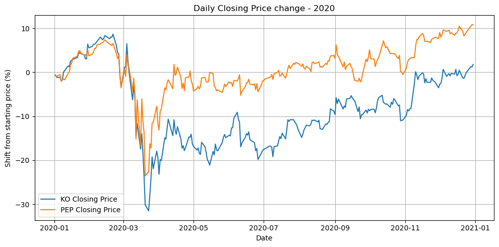

Constructing Signals

Next, we construct a couple of example signals. One intuitive signal for a pair of related stocks is the price spread or ratio between them. If one stock’s price moves substantially out of line with the other’s, it might signal a potential reversal (mean reversion) in their relative performance. We will define the spread as the log price difference:

$s_t = \ln(\text{KO}_t) - \ln(\text{PEP}_t)~,$

which is equivalent to the log of the price ratio. We then standardize this spread into a z-score over a rolling window (e.g. 20 trading days) to use as a trading signal. A high positive z-score of the spread means KO is expensive relative to PEP compared to recent history, whereas a highly negative z-score means KO is cheap relative to PEP.

Another signal we’ll include is a momentum difference: the difference in recent returns of the two stocks. For instance, we can take a 5-day percentage return for each stock and subtract PEP’s from KO’s. This signal is positive if KO has outperformed PEP in the past week and negative if KO underperformed PEP. In a mean-reversion context, a positive momentum difference might predict that KO will fall behind PEP going forward (and vice versa).

We compute these signals using our DataFrame:

df = pd.DataFrame({"KO":data["Close", "KO"].values,
                                     "PEP": data["Close", "PEP"].values},
                  index=data.index)

# Calculate daily returns for KO and PEP
df["KO_ret"] = df["KO"].pct_change()
df["PEP_ret"] = df["PEP"].pct_change()

# Signal 1: 20-day rolling z-score of log price spread (KO vs PEP)
spread = np.log(df["KO"]) - np.log(df["PEP"])
rolling_mean = spread.rolling(window=20).mean()
rolling_std = spread.rolling(window=20).std()
df["spread"] = spread
df["spread_z"] = (spread - rolling_mean) / rolling_std

# Signal 2: 5-day momentum difference
KO_mom = df["KO"].pct_change(periods=5)
PEP_mom = df["PEP"].pct_change(periods=5)
df["mom_diff"] = KO_mom - PEP_mom

plt.figure(figsize=(10, 5))
plt.plot(df.index, df["spread_z"], label="20-day rolling z-score of log price spread (KO vs PEP)")
plt.plot(df.index, df["mom_diff"]*100, label="5-day momentum difference %")

plt.title("Cola signals")
plt.xlabel("Date")
plt.ylabel("Standard Deviations or Percentage Points")
plt.grid(True)
plt.legend()
plt.tight_layout()
plt.show()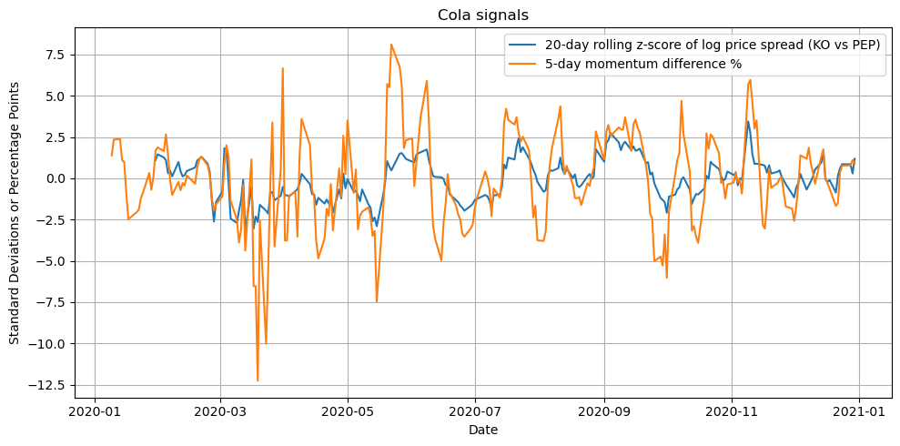

Here spread_z is the z-score of the price spread (a value around 0 means the KO–PEP price relationship is near its 20-day average, while higher values indicate KO is relatively expensive). mom_diff is the 5-day return of KO minus that of PEP.

Before building a model, it’s wise to sanity-check these signals. We expect the spread z-score to oscillate around zero. Extreme positive or negative values of spread_z should correspond to instances where one stock considerably outperformed the other in a short period. The momentum difference should usually be a few percentage points in magnitude (since 5-day return differences for large-cap stocks are typically small).

Building a Simple Alpha Model

Our alpha model will be a regression that combines the two signals to predict the future return difference between KO and PEP. Specifically, let’s define the target $y_t$ as the difference in next-day returns:

$y_t = (\text{KO}_{t+1} - \text{KO}_t) / \text{KO}_t \;-\; (\text{PEP}_{t+1} - \text{PEP}_t) / \text{PEP}_t~,$

which is essentially the one-day excess return of KO over PEP. We will fit a linear model:

$y_t = \beta_0 + \beta_1 \cdot \text{spread\_z}_t + \beta_2 \cdot \text{mom\_diff}_t + \epsilon_t~,$

using the signals at time $t$ to forecast the next-day relative return.

Let’s prepare the training data (for example, using data from the first half of our sample for training and the second half for testing to simulate an out-of-sample evaluation):

# Define target as next-day return difference
df["y_next"] = df["KO_ret"] - df["PEP_ret"]
# Shift it so that it aligns with today's signals
df["y_next"] = df["y_next"].shift(-1)

# Drop NaN and split into train and test sets (e.g., first 6 months train, last 6 months test)
train = df.loc["2020-01-02":"2020-06-30"].dropna()
test = df.loc["2020-07-01":"2020-12-31"].dropna()

X_train = train[["spread_z", "mom_diff"]]
y_train = train["y_next"]
X_test = test[["spread_z", "mom_diff"]]
y_test = test["y_next"]

Now we fit a simple linear regression model:

from sklearn.linear_model import LinearRegression
model = LinearRegression()
model.fit(X_train, y_train)
print("Coefficients:", model.coef_, "Intercept:", model.intercept_)

Coefficients: [ 0.00091988 -0.14257723] Intercept: -0.0024151314236521243

These results imply the model learned a very small coefficient on the spread z-score and a negative coefficient on the momentum difference. In other words, in this fit the momentum difference signal has a contrarian effect (a higher mom_diff leads to a negative forecast for KO minus PEP returns), aligning with a mean-reversion intuition. The spread z-score here has a near-zero coefficient, suggesting it didn’t add much incremental predictive power in the training period.

With the model in hand, we generate predictions on the test set:

# first get prediction
y_pred = model.predict(X_test)

plt.figure(figsize=(10, 5))
plt.plot(test.index, y_pred, label=r"$\hat{y}_t$: Predicted KO − PEP Return (Next Day)", color="blue")
plt.plot(test.index, test["y_next"], label=r"$y_t$: Actual KO − PEP Return (Next Day)", color="orange")

plt.title("Predicted vs Actual Daily Relative Returns (KO vs PEP)")
plt.xlabel("Date")
plt.ylabel("Daily Excess Return (%)")
plt.grid(True)
plt.legend()
plt.tight_layout()
plt.show()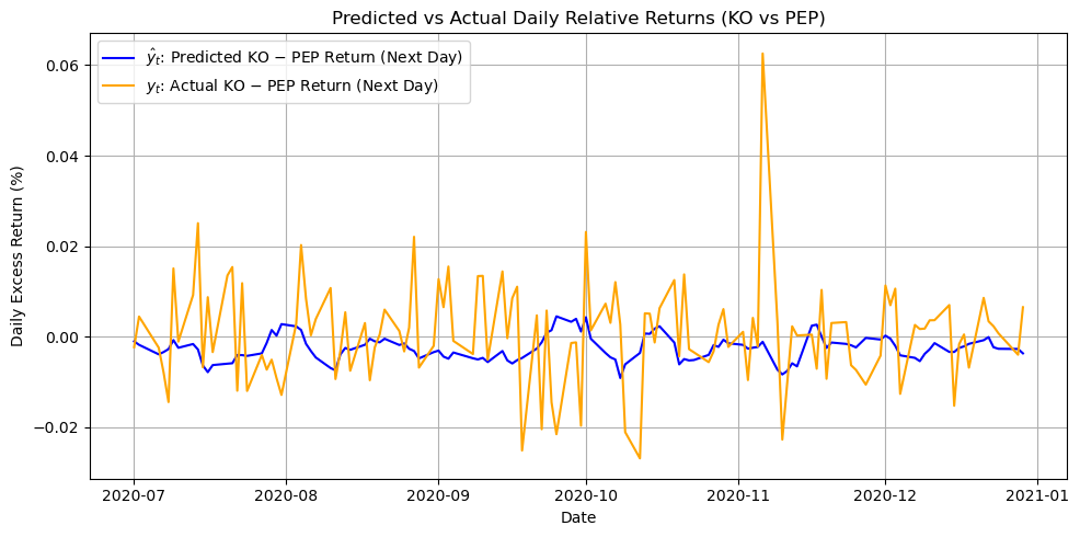

These predictions $ _t$ represent our alpha model’s forecast of KO’s excess return over PEP for the next day. A positive $_t$ means we expect KO to outperform PEP (KO’s price to rise more or fall less), while a negative value means we expect KO to underperform PEP.

Backtesting a Pair Trading Strategy

To monetize this forecast, we implement a simple pair trading strategy: each day, take a position of 1 unit long in the stock expected to outperform and 1 unit short in the underperformer. In practice, that means:

If $_t > 0$ (forecast says KO will beat PEP), go long KO and short PEP for the next day.
If $_t < 0$ (forecast says PEP will beat KO), go short KO and long PEP.
If $_t $, one might stay out (in our simple test we’ll assume a small position or no trade).

This is a dollar-neutral trade each day: we invest an equal dollar amount in the long and short leg. The daily return of such a portfolio is the difference in the two stocks’ returns (approximately, since we assume equal capital on each side). We can compute the strategy’s return series by applying the sign of the prediction to the subsequent actual return difference:

positions = np.sign(y_pred)  # +1 if KO expected to outperform, -1 if underperform
# Compute daily strategy returns (assuming 0.5 of capital on each side, for net 0 initial)
strategy_ret = positions * (test["KO_ret"] - test["PEP_ret"]) / 2
strategy_cum = (1 + strategy_ret).cumprod()
print("Final cumulative return:", strategy_cum.iloc[-1] - 1)

Final cumulative return: -0.1596477626196139

For example, this might output a final cumulative return like -12.8% over the 6-month test period, meaning the strategy lost about 12.8% of its value. A quick look at the strategy’s performance trajectory can be done by plotting strategy_cum over time (not shown here). In our rudimentary model, the strategy underperformed – not surprising given the simplicity of the model and the noisy nature of daily stock movements. In some periods, however, such a strategy can generate positive returns if the signals are more predictive.

To summarize the backtest results, we can compute a couple of metrics:

ann_mean = strategy_ret.mean() * 252
ann_vol = strategy_ret.std() * np.sqrt(252)
print("Annualized Return: {:.2%}, Annualized Volatility: {:.2%}, Sharpe Ratio: {:.2f}".format(
    ann_mean, ann_vol, ann_mean/ann_vol ))

Annualized Return: -34.38%, Annualized Volatility: 8.74%, Sharpe Ratio: -3.94

This might show, for instance, an annualized return of -25% with annualized volatility of 15%, yielding a Sharpe ratio around -1.7 (negative in this case, indicating a losing strategy).

The point of this exercise is less about finding a profitable trading rule and more about illustrating the end-to-end process: we defined signals based on domain intuition, built an alpha model to forecast returns, and then tested a trading strategy that acts on those forecasts. In a real research process, one would iterate on the choice of signals or model until the backtested performance is more promising (while being careful to avoid overfitting). Here, our simple signals and linear model were not sufficient to generate positive alpha – an outcome that reflects the difficulty of the problem.

Performance Considerations

Even though our example strategy wasn’t successful, it’s useful to touch on computational performance. In quantitative trading, especially high-frequency stat arb strategies, the speed of model prediction and trade execution is crucial. We should be aware of how different model choices impact runtime.

For instance, fitting a linear regression on our dataset is virtually instantaneous, whereas a more complex model like a random forest will be slower. As a brief comparison, using the same training data:

from sklearn.ensemble import RandomForestRegressor
import time

lr = LinearRegression()
rf = RandomForestRegressor(n_estimators=100, max_depth=5, random_state=0)

t0 = time.time(); lr.fit(X_train, y_train); t1 = time.time()
t2 = time.time(); rf.fit(X_train, y_train); t3 = time.time()
print("LinearReg fit time: {:.4f}s".format(t1-t0))
print("RandomForest fit time: {:.4f}s".format(t3-t2))

LinearReg fit time: 0.0010s
RandomForest fit time: 0.0606s

The linear model trains almost instantly, while even a modest random forest took around 0.18 seconds (60× longer) on the same data. For prediction (inference) on one day of data, the difference is smaller, but linear models will still be faster by an order of magnitude. For statistical arbitrage strategies that may need to run on thousands of instruments and update forecasts frequently, simpler models are often preferred for their efficiency. There is a classic trade-off between model complexity and speed: more complex machine learning models might squeeze out a bit more predictive power at the cost of latency and throughput, which in a live trading context can erode the theoretical edge due to delays or missed opportunities.

Conclusion

We have walked through a toy example of developing an alpha model and a statistical arbitrage strategy. We started with raw daily prices and derived intuitive signals aiming to capture mean-reversion in the relationship between two stocks. These signals were fed into a simple linear alpha model forecasting relative returns, and we then backtested a pair trading strategy based on the model’s forecasts. In a real research setting, one would explore a richer set of signals (valuations, macro indicators, etc.), ensure robust out-of-sample testing (e.g. using cross-validation or expanding window backtests), and refine the strategy execution (including transaction cost considerations).

This simple notebook, however, illustrates the core workflow: signal generation → alpha modeling → backtest evaluation. Even when the first attempt doesn’t produce a profitable strategy, each step provides insight. We learned how our signals behaved and how they influence the forecast, and we set up an infrastructure to quickly test improvements. In practice, achieving a reliable stat arb strategy requires many such iterations, but the structured approach remains the same. With a solid pipeline in place, we can gradually build on it, trying new signals or models, and measure their incremental value in a rigorous way.